
Wednesday, August 28, 2013
그림으로 이해하는 닥터 배의 술술 보건의학통계
Tuesday, August 20, 2013
interval tree
SnpEff (https://www.landesbioscience.com/journals/fly/2011FLY0072R1.pdf)
: SNPs, MNPs (multiple nucleotide polymorphism), InDels 등을 annotation 할때 쓰는 프로그램
위 논문의 내용은 말그대로 variant를 찾고 나서 그 뒤에 variant에 대한 annotation을 해주는 프로그램인 SnpEff를 사용하여 Drosophila의 strain의 SNP, MNPs, InDels 등을 annotation 한 논문.
프로그램 차원에서 보면 중요한 keyword는
""interval forest, which is a hash of interval trees indexed by chromosome"".
Interval Trees
http://www.dgp.utoronto.ca/people/JamesStewart/378notes/22intervals/
interval 은 정수 쌍을 의미([a,b] such that a<b)
elementary interval은 interval의 end point (integer) 에 의해 생기는 partition을 의미.
예를 들어 interval x=[10,20],y=[15,25],z=[18,22] 가 있을때 아래 그림과 같이 7개의 elementary interval이 생긴다.
 이 interval들을 저장하기 위한 자료 구조로 BST(binary search tree)를 이용한다.
일단 elementary interval을 저장할 수 있는 자료 구조로 아래와 같은 tree 생성.
 각 leaf node는 elementary interval을 나타나게 된다. 여기서 interval의 정보를 넣는 방법은..
단순하게 생각하면 아래와 같을 수 있다.
 문제는 too much memory !
그래서 아래와 같은 두가지 조건으로 internal node 까지 사용한다.
1.node의 범위가 interval 에 완전히 포함되고 2.그 node의 parent node 범위는 interval을 벗어나면 그 node에 interval 을 저장. 그러면 아래와 같이 interval을 저장하게 된다.

좀더 복잡한 예제를 보자면 아래와 같은 작곡가의 일생을 interval로 tree 를 만들면
 아래와 보는 바와 같다.

여기서 문제. 1910년 경에 살았던 작곡가는 누구인가라는 문제에 대한 해답은 어떻게 찾는가?
1910을 span 하고 있는 leaf에 담긴 interval이 그 해답. 곧 A,B. 그런데 만약 문제가 1880년 경이라면? 1880을 span 하고 있는 leaf는 아무 interval도 포함하고 있지 않다.
그래서 정확하게 해당 interval을 찾는 과정은 해당 년도를 포함하고 있는 leaf에서부터 root 까지의 interval을 다 찾는 것. 다르게 이야기 하면 root 에서 해당 년도를 span 하고 있는 leaf를 찾아가면서 각 internal node의 interval을 다 찾으면 되는 것. 곧 root-to-leaf path finding문제가 된다.
Interval Tree Code for Python
http://blog.nextgenetics.net/?e=45
Return to Paper
Each interval tree is composed of nodes. Each node has five elements (i) a center point, (ii) a pointer to a node having all intervals to the left of the center, (iii) a pointer to a node having all intervals to the right of the center, (iv) all intervals overlapping the center point sorted by start position, and (v) all intervals overlapping the center point, sorted by end position
: SNPs, MNPs (multiple nucleotide polymorphism), InDels 등을 annotation 할때 쓰는 프로그램
위 논문의 내용은 말그대로 variant를 찾고 나서 그 뒤에 variant에 대한 annotation을 해주는 프로그램인 SnpEff를 사용하여 Drosophila의 strain의 SNP, MNPs, InDels 등을 annotation 한 논문.
프로그램 차원에서 보면 중요한 keyword는
""interval forest, which is a hash of interval trees indexed by chromosome"".
Interval Trees
http://www.dgp.utoronto.ca/people/JamesStewart/378notes/22intervals/
interval 은 정수 쌍을 의미([a,b] such that a<b)
elementary interval은 interval의 end point (integer) 에 의해 생기는 partition을 의미.
예를 들어 interval x=[10,20],y=[15,25],z=[18,22] 가 있을때 아래 그림과 같이 7개의 elementary interval이 생긴다.
일단 elementary interval을 저장할 수 있는 자료 구조로 아래와 같은 tree 생성.

단순하게 생각하면 아래와 같을 수 있다.

그래서 아래와 같은 두가지 조건으로 internal node 까지 사용한다.
1.node의 범위가 interval 에 완전히 포함되고 2.그 node의 parent node 범위는 interval을 벗어나면 그 node에 interval 을 저장. 그러면 아래와 같이 interval을 저장하게 된다.

좀더 복잡한 예제를 보자면 아래와 같은 작곡가의 일생을 interval로 tree 를 만들면

여기서 문제. 1910년 경에 살았던 작곡가는 누구인가라는 문제에 대한 해답은 어떻게 찾는가?
1910을 span 하고 있는 leaf에 담긴 interval이 그 해답. 곧 A,B. 그런데 만약 문제가 1880년 경이라면? 1880을 span 하고 있는 leaf는 아무 interval도 포함하고 있지 않다.
그래서 정확하게 해당 interval을 찾는 과정은 해당 년도를 포함하고 있는 leaf에서부터 root 까지의 interval을 다 찾는 것. 다르게 이야기 하면 root 에서 해당 년도를 span 하고 있는 leaf를 찾아가면서 각 internal node의 interval을 다 찾으면 되는 것. 곧 root-to-leaf path finding문제가 된다.
Interval Tree Code for Python
http://blog.nextgenetics.net/?e=45
Return to Paper
Each interval tree is composed of nodes. Each node has five elements (i) a center point, (ii) a pointer to a node having all intervals to the left of the center, (iii) a pointer to a node having all intervals to the right of the center, (iv) all intervals overlapping the center point sorted by start position, and (v) all intervals overlapping the center point, sorted by end position
Monday, August 19, 2013
adaboost
Top 10 Algorithms in Data Mining 중 하나인 adaboost 에 대해 알아본다. 이후 가능하다면 adaboost를 적용한 논문인 defuse에 대한 요약을 하도록 하겠다 (아래 내용은 책 "Machine Learning in Action" 을 기반으로 한다).
다양한 classifier를 결합하는 방법을 ensemble method 혹은 meta algorithm이라 한다.
이런 meta algorithm 에는 bagging, random forests, boosting 방법등이 있다.
adaboost 는 adaptive boost의 줄임말로 boosting 의 한가지 유형이다.


stumpClassify는 데이터(dataMatrix)를 특정 feature (dimen), threshold value (threshVal) 그리고 그 threshold 를 기준으로 큰 값 혹은 작은 값인지를 판단하는 threshIneq를 가지고 분류하는 기능을 한다.

buildStump 는 data array (dataArr), classLabels와 가중치 벡터 (D) 를 받아서 분류를 가장 잘하는 feature (dim) 와 특정 값 (thresh)과 그것에 대한 기준(ineq) 을 찾는 역할(stump 생성)을 한다.

adaBoostTrainDS 는 data array (dataArr), classLabels와 iteration 횟수 (numIt) 를 받아서 numIt 횟수만큼(혹은 errorRate가 0일 때까지) 반복을 하면서 가중치 벡터 (D)를 갱신해가며 buildStump를 이용해서 얻은 최적의 stump 들을 리스트 weakClassArr 에 쌓아 놓는다.
위에서 D를 어떻게 갱신해가는가를 보면 buildStump가 만든 stump가 맞으면 D를 줄이고 틀리면 D 를 늘리는 방향으로 갱신하는데 이때 줄이고 늘리는 정도가 그 stump의 정확도에 비례한다. 곧 정확도가 높을 수록 맞춘 예의 D는 크게 줄이고 틀린 예의 D는 크게 늘린다.

adaClassify는 datToClass는 분류하고자 하는 새로운 데이터, classifierArr는 adaBoostTrainDS 통해 얻은 weak classifier array (weakClassArr) 를 인자로 받는다.
adaBoostTrainDS 통해 얻은 weak classifier array (weakClassArr)를 이용하여 데이터(dataToClass) 를 분류한다. 이 때 weakClassArr에 있는 classifier를 하나씩 이용해서 분류한 값과 alpha 값의 곱을 누적시켜서 최종적인 분류를 하게 된다.
정리를 하자면 adaboost는 weak classifier 들의 집합을 만들고 그 weak classifier들의 분류값을 그 classifier의 정확도에 기반한 가중치(alpha) 의 곱의 합으로 새로운 데이터를 분류하게 된다.
다양한 classifier를 결합하는 방법을 ensemble method 혹은 meta algorithm이라 한다.
이런 meta algorithm 에는 bagging, random forests, boosting 방법등이 있다.
adaboost 는 adaptive boost의 줄임말로 boosting 의 한가지 유형이다.
stumpClassify는 데이터(dataMatrix)를 특정 feature (dimen), threshold value (threshVal) 그리고 그 threshold 를 기준으로 큰 값 혹은 작은 값인지를 판단하는 threshIneq를 가지고 분류하는 기능을 한다.
buildStump 는 data array (dataArr), classLabels와 가중치 벡터 (D) 를 받아서 분류를 가장 잘하는 feature (dim) 와 특정 값 (thresh)과 그것에 대한 기준(ineq) 을 찾는 역할(stump 생성)을 한다.
adaBoostTrainDS 는 data array (dataArr), classLabels와 iteration 횟수 (numIt) 를 받아서 numIt 횟수만큼(혹은 errorRate가 0일 때까지) 반복을 하면서 가중치 벡터 (D)를 갱신해가며 buildStump를 이용해서 얻은 최적의 stump 들을 리스트 weakClassArr 에 쌓아 놓는다.
위에서 D를 어떻게 갱신해가는가를 보면 buildStump가 만든 stump가 맞으면 D를 줄이고 틀리면 D 를 늘리는 방향으로 갱신하는데 이때 줄이고 늘리는 정도가 그 stump의 정확도에 비례한다. 곧 정확도가 높을 수록 맞춘 예의 D는 크게 줄이고 틀린 예의 D는 크게 늘린다.
adaClassify는 datToClass는 분류하고자 하는 새로운 데이터, classifierArr는 adaBoostTrainDS 통해 얻은 weak classifier array (weakClassArr) 를 인자로 받는다.
adaBoostTrainDS 통해 얻은 weak classifier array (weakClassArr)를 이용하여 데이터(dataToClass) 를 분류한다. 이 때 weakClassArr에 있는 classifier를 하나씩 이용해서 분류한 값과 alpha 값의 곱을 누적시켜서 최종적인 분류를 하게 된다.
정리를 하자면 adaboost는 weak classifier 들의 집합을 만들고 그 weak classifier들의 분류값을 그 classifier의 정확도에 기반한 가중치(alpha) 의 곱의 합으로 새로운 데이터를 분류하게 된다.
Tuesday, August 13, 2013
structure software
STRUCTURE 프로그램은 unlinked marker (recombinant allele의 frequency가 50% 이면 unlinked, 곧 marker 간의 거리가 먼, 2.0 version 이후로는 weakly linked markder도 다룬다고 함) 의 genotype data를 가지고 model-based clustering method를 이용하여 population structure를 추정하는 프로그램. (http://pritch.bsd.uchicago.edu/structure.html). 이 posting 에서는 우선적으로 manual(http://pritch.bsd.uchicago.edu/structure_software/release_versions/v2.3.4/structure_doc.pdf) 내용을 기반으로 하고 가능하다면 논문(http://pritch.bsd.uchicago.edu/publications/structure.pdf) 도 cover 해보고자 한다
introduction으로 홍창범씨의 블로그의 예제 (http://hongiiv.tistory.com/610) 를 실행해보는 것이 좋다.
how to format the data files

맨 첫줄(underbar 위에 있는 것)은 이해를 돕고자 넣은 것이고 그 다음 line 부터가 structure의 input format이다.
아래는 row 1부터 row 별 설명이다.
how to choose appropriate models
Ancestry models
how to interpret the results
how to estimate of K (the number of populations)
introduction으로 홍창범씨의 블로그의 예제 (http://hongiiv.tistory.com/610) 를 실행해보는 것이 좋다.
how to format the data files

아래는 row 1부터 row 별 설명이다.
- Marker Names
- Recessive Alleles
- Inter-Marker Distances
- Phase Information
- Individual/Genotype data
- Label
- PopData
- PopFlag
- LocData
- Phenotype
- Extra Columns
- Genotype Data
how to choose appropriate models
Ancestry models
- No admixture model : individuals are discretely from one population or another : 각 개인이 온전히 하나의 population 에서부터만 유래한 것 (population이 하나라는 의미가 아니라 각 개인의 genome이 여러 population 이 섞인 것이 아니라 딱 하나의 population 에서부터 왔다는 의미). 이 경우 individual i가 population k에 속할 posterior probability (P(model|data))를 report하게 된다.
- Admixture model : each individual draws some fraction of his/her genome from each of the K populations : 각 개인의 genome이 여러 population이 섞인 경우.
- Linkage model : like the admixture model, but linked loci are more likely to come from the same population :
- Using prior population information
- LOCPRIOR model
- USEPOPINFO model
- USEPOPINFO model
Allele frequency models
- Estimating λ
- Correlated allele frequencies model
how to interpret the results
how to estimate of K (the number of populations)
something about population genomics
다음은 Resequencing of 31 wild and cultivated soybean genomes identifies patterns of genetic diversity and selection 이라는 논문의 이해를 돕기 위한 background knowledge를 위함이다.
먼저 용어 이해부터...
"""We identified a high level of linkage disequilibrium in the soybean genome, suggesting that marker-assisted breeding of soybean will be less challenging than map-based cloning"""
"""We identified a set of 205,614 tag SNPs that may be useful for QTL mapping"""
QTL mapping : http://graphy21.blogspot.kr/2013/08/qtl-mapping.html
"""From this analysis, we identified a total of 6,318,109 SNPs and 186,177 PAVs"""
PAV(presence-absence variation) : describe sequences that are present in one genome but entirely missing in the other genome.
"""We constructed a rooted phylogenetic tree using Lotus japonicus as the outgroup"""
outgroup : 3개 이상의 monophyletic group 혹은 species들의 evolutionary relationship을 결정할 때 reference group 혹은 species로 사용되는 monophyletic group 혹은 species(monophyletic 이라 함은 하나의 ancestral species고 나머지 species는 그것으로 부터 파생된 group). group들 중 the most recent common ancestor (=root) 로 부터 가장 먼저 branching 된 group. rooted tree를 구축할때 outgroup을 이용한다. 곧 unrooted tree를 구축했으면(http://graphy21.blogspot.kr/2013/08/coursera-computational-molecular.html 참조) outgroup이 정해지면 rooted tree로 transform이 가능.
 transform unrooted tree to rooted tree with outgroup
아래 내용은 http://cabbagesofdoom.blogspot.kr/2012/06/how-to-root-phylogenetic-tree.html 의 내용에 기반한다.

"""Using the Baysesian clustering program STRUCTURE, with K changing progressively from 2-7"""
STRUCTURE : http://graphy21.blogspot.kr/2013/08/structure-software.html 참조
"""Whole-genome SNP analysis, using the parameter Θπ, also identified a lower level of genetic diversity in cultivated soybeans compared to wild soybeans"""
""" Calculation of the divergence index(Fst) value between wild and cultivated soybeans allowed us to identify genomic regions of large Fst value, which signified areas having a high degree of diversification between wild and cultivated soybeans"""
Fst는 total population 내의 subpopulation 간에 differentiation 정도를 나타내기 때문에, wild와 cultivated soybean의 genomic region 별 Fst를 구함으로 해서 두 그룹간에 분리가 되는 genomic region을 찾기 위함.
Fst(fixation index) : developed as a special case of Wright's F-statistics
Fst가 0 이면 no divergence between population (interbreeding freely), 1이면 complete isolation. 아래 F-statistics 참조.
Inbreeding coeffiecient : subpopulation 에서의 non-random mating 에 의한 heterozygosity가 줄어든 정도를 나타냄. FIS로 표시하나 단순하게 F로 대신 표현하기도 한다(상황에 따라 구분을 잘해야 한다, 아래 F-statistics 에서는 F와 FIS를 구분하여 사용).
HS = mean expected heterozygosity within random mating subpopulations
아래 F-statistics 참조
-1에서 1 까지 값을 갖으며 -1은 모든 individual이 heterozygous 할때, 1은 heterozygous한 individual 이 하나도 없음을 의미(0은 observed와 expected의 갯수가 동일한 상황).
F-statistics : statistically expected level of heterozygosity in population. Hardy-Weinberg expectation과 비교했을 때 heterozygosity 가 적어진 정도를 나타내는 값.
특정 genomic locus 에 A와 a allele 두 가지가 있다고 할 때, F의 계산은 아래와 같다.
 f(Aa)는 heterozygous genotype의 frequency. 곧 1- observed / expected의 값이 F-statistics. F의 수치가 높으면 observed frequency가 expected frequency에 비해 작다는 것(차이가 크다는 것).
예를 들어 보면

 F-statistics 에는 어떤 population structure 의 level에 초점을 두느냐에 따라 FIS, FST, FIT로 구분된다.
I는 individual을 S는 subpopulation을 T는 total population을 의미.
FIS 와 FIT는 위의 F-statistics 방법 대로 계산하고 FST는 아래 식을 이용하여 계산.
 FST는 Wahlund effect 에 의한 것이고 FIS는 inbreeding에 의한것.
""""""""""""""""""""""""""""""""""""""""""""""""""""""""""""""""""""""""""""""""""""""""""""""""""""""""""""""""""""""""""""""""
FIS, FST, FIT 이부분의 이해를 돕고자 아래 내용을 참고한다.
http://www.library.auckland.ac.nz/subject-guides/bio/pdfs/733Pop-g-stats2.pdf
 H는 heterozygosity를 의미.
HI = mean observed heterozygosity per individual within subpopulations
HS = mean expected heterozygosity within random mating subpopulations
Wright에 의하면 Fst의 값에 따라 해석하는 guideline을 제시했는데..
0.00~0.05 : little genetic differentiation, 0.05~0.15 : moderate, 0.15~0.25 : great, 0.25~ : very great
위의 내용은 allele frequency에 기반한 Fst 계산법.
DNA Sequence Data 를 기반한 Fst 계산법을 알아본다 (여러가지가 있는데 그 중 단순하고 이해가 될만한 것으로).
1982년 Nei 에 의해 고안된 것으로 H (heterozygosity) 대신 nucleotide diversity (π) 를 사용한다.
 πT는 total population 에서의 nucleotide diversity를 의미하며, pi, pj는 haplotype i와 haplotype j의 frequency를 의미, πij 는 haplotype i와 haplotype j 의 genetic distance(단순 DNA difference proportion일 수도 있고, Juke-Cantor 방법 혹은 Kimura 2- parameter 의 substitution rate에 의한 distance 일 수 있다) 를 의미.
 πT와 더불어 subpopulation 내의 average necleotide diversity인 πS-bar를 계산하게 되면 위 식으로 Fst-like nucleotide measure of subpopulation differentiation 인 γst를 구할수 있다(πB 는 average nucleotide diversity between subpopulations).

위 식 이외의 Fst 계산 방법

"""""""""""""""""""""""""""""""""""""""""""""""""""""""""""""""""""""""""""""""""""""""""""""""""""""""""""""""""""""""""""""""
Wahlund effect : 한 population 안에 여러 subpopulation이 섞여 있음으로 해서 heterozygosity 가 적어지는 현상. 예를 들어 한 population 안에 두개의 subpopulation이 있다고 할 때 각 subpopulation이 HW equilibrium 상태에 있다고 하면 아래와 같이 두 subpopulation의 같은 allele의 frequency가 동일하지 않는이상 heterozygosity의 수가 적게 나타나는 현상이 생긴다.

Linkage disequilibrium (LD) : 두 loci A,B가 있고 각 locus 마다 2개의 allele type이 있을 때
위의 왼쪽 table과 같이 haplotype의 frequency가 있을 때 각 locus의 allele의 frequency를 위의 오른쪽 table과 같이 계산 가능하다. 위 allele frequency를 가지고 두 loci가 독립이다라는 가정하에 haplotype을 다시 계산할수 있다(x11 = p1*q1 등등).
 이때 이 observed frequency와 독립이라는 가정하의 haplotype frequency의 차이를 linkage disequilibrium (LD) 이라고 하며 이 값이 0 이면 'linkage equilibrium' 아니면 'linkage disequilibrium' 이라 한다 (D 값을 x12로 계산하려면 p1q2 - x12 = D, 이는 x11 + x12 = p1, 곧 x11 = p1 - x12, 그러므로 x11 - p1q1 = p1 - x12 - p1q1 = p1(1-q1) - x12 = p1q2 - x12 = D).
이 D 값은 allele frequency 에 dependent 하기 때문에(이것의 정확한 의미는 이해가 되지 않음..) D' 혹은 r (correlation coefficient) 를 사용.
 혹은
혹은 
http://en.wikipedia.org/wiki/Linkage_disequilibrium 뒷 부분을 보게 되면 HLA를 이용한 LD-test 예제가 나온다(예상되기로는 A1과 B8의 유전자가 dominant 라 gfi를 계산할때 root를 씌어줌). D를 구하고 D의 SE (standard error) 를 구해서 t-statistics로 변형 후 검정
Hardy-Weinberg expectation : Hardy-Weinberg principle이 어떠한 진화적인 압박이나 영향이 없을 때 allele 이나 genotype의 frequency가 일정하게 유지된다라는 것. 가장 simple 한 예가 2개의 allele을 갖는 locus 의(A,a 라고 가정), frequency of A allele f(A) = p 과 f(a) = q 일 때 expected genotype frequencies인 f(AA)=p^2, f(aa) = a^2, f(Aa) = Aa 가 된다. 그리고 다음 세대를 위한 gametes가 random하다는 가정하에 다음 세대의 A와 a 의 frequency는 동일하게 되고 마찬가지로 genotype의 frequency 역시 동일하게 된다.
먼저 용어 이해부터...
"""We identified a high level of linkage disequilibrium in the soybean genome, suggesting that marker-assisted breeding of soybean will be less challenging than map-based cloning"""
"""We identified a set of 205,614 tag SNPs that may be useful for QTL mapping"""
QTL mapping : http://graphy21.blogspot.kr/2013/08/qtl-mapping.html
"""From this analysis, we identified a total of 6,318,109 SNPs and 186,177 PAVs"""
PAV(presence-absence variation) : describe sequences that are present in one genome but entirely missing in the other genome.
"""We constructed a rooted phylogenetic tree using Lotus japonicus as the outgroup"""
outgroup : 3개 이상의 monophyletic group 혹은 species들의 evolutionary relationship을 결정할 때 reference group 혹은 species로 사용되는 monophyletic group 혹은 species(monophyletic 이라 함은 하나의 ancestral species고 나머지 species는 그것으로 부터 파생된 group). group들 중 the most recent common ancestor (=root) 로 부터 가장 먼저 branching 된 group. rooted tree를 구축할때 outgroup을 이용한다. 곧 unrooted tree를 구축했으면(http://graphy21.blogspot.kr/2013/08/coursera-computational-molecular.html 참조) outgroup이 정해지면 rooted tree로 transform이 가능.

아래 내용은 http://cabbagesofdoom.blogspot.kr/2012/06/how-to-root-phylogenetic-tree.html 의 내용에 기반한다.

"""Using the Baysesian clustering program STRUCTURE, with K changing progressively from 2-7"""
STRUCTURE : http://graphy21.blogspot.kr/2013/08/structure-software.html 참조
"""Whole-genome SNP analysis, using the parameter Θπ, also identified a lower level of genetic diversity in cultivated soybeans compared to wild soybeans"""
""" Calculation of the divergence index(Fst) value between wild and cultivated soybeans allowed us to identify genomic regions of large Fst value, which signified areas having a high degree of diversification between wild and cultivated soybeans"""
Fst는 total population 내의 subpopulation 간에 differentiation 정도를 나타내기 때문에, wild와 cultivated soybean의 genomic region 별 Fst를 구함으로 해서 두 그룹간에 분리가 되는 genomic region을 찾기 위함.
Fst(fixation index) : developed as a special case of Wright's F-statistics
Fst가 0 이면 no divergence between population (interbreeding freely), 1이면 complete isolation. 아래 F-statistics 참조.
Inbreeding coeffiecient : subpopulation 에서의 non-random mating 에 의한 heterozygosity가 줄어든 정도를 나타냄. FIS로 표시하나 단순하게 F로 대신 표현하기도 한다(상황에 따라 구분을 잘해야 한다, 아래 F-statistics 에서는 F와 FIS를 구분하여 사용).
FIS = (HS - HI) / HS
HI = mean observed heterozygosity per individual within subpopulationsHS = mean expected heterozygosity within random mating subpopulations
아래 F-statistics 참조
-1에서 1 까지 값을 갖으며 -1은 모든 individual이 heterozygous 할때, 1은 heterozygous한 individual 이 하나도 없음을 의미(0은 observed와 expected의 갯수가 동일한 상황).
F-statistics : statistically expected level of heterozygosity in population. Hardy-Weinberg expectation과 비교했을 때 heterozygosity 가 적어진 정도를 나타내는 값.
특정 genomic locus 에 A와 a allele 두 가지가 있다고 할 때, F의 계산은 아래와 같다.
예를 들어 보면
I는 individual을 S는 subpopulation을 T는 total population을 의미.
FIS 와 FIT는 위의 F-statistics 방법 대로 계산하고 FST는 아래 식을 이용하여 계산.
""""""""""""""""""""""""""""""""""""""""""""""""""""""""""""""""""""""""""""""""""""""""""""""""""""""""""""""""""""""""""""""""
FIS, FST, FIT 이부분의 이해를 돕고자 아래 내용을 참고한다.
http://www.library.auckland.ac.nz/subject-guides/bio/pdfs/733Pop-g-stats2.pdf

HI = mean observed heterozygosity per individual within subpopulations
HS = mean expected heterozygosity within random mating subpopulations
HT = expected heterozygosity in random mating total population
위의 식을 보면 subpopulation이 두개 이상인데 어떻게 하나의 HI,HS 를 선택할 수 있나 라는 생각이 들 수 있는데 저 값들은 subpopulation의 값들의 평균 값임을 기억하자. - inbreeding coefficient = FIS = (HS - HI) / HS
- subpopulation 에서의 non-random mating 에 의한 H의 reduction 정도를 나타냄
- subpopulation 내에서 genetic inbreeding의 정도
- -1 <= FIS <= 1 (-1: all H, 1: no H)
- fixation index = FST = (HT - HS) / HT
- total population 대비해서 subpopulation의 H 의 reduction 정도를 나타냄 (genetic drift에 의한)
- subpopulation 간의 genetic differentiation을 의미
- 0 <= FST <= 1 (0: no differentiation, 1: complete differentiation between subpopulations)
- 결국 위 식은 1 - HS / HT 인데, HS는 subpopulation의 expected H의 평균값. 곧 Fst가 0 이란 의미는 subpopulation의 expected H의 평균값이 total population의 expected H와 같다는 것. 곧 subpopulation 간의 heterozygosity의 차이가 없다는 의미.
- 예를 들어 Fst가 0.39가 나왔다면 total genetic variation의 39%는 subpopulation 간에 의한 것이고 61 %는 within subpopulation의 variation에 의한 것
- overall fixation index = FIT = (HT - HI) / HT
- total population 에서의 H의 reduction 정도를 나타냄
Wright에 의하면 Fst의 값에 따라 해석하는 guideline을 제시했는데..
0.00~0.05 : little genetic differentiation, 0.05~0.15 : moderate, 0.15~0.25 : great, 0.25~ : very great
위의 내용은 allele frequency에 기반한 Fst 계산법.
DNA Sequence Data 를 기반한 Fst 계산법을 알아본다 (여러가지가 있는데 그 중 단순하고 이해가 될만한 것으로).
1982년 Nei 에 의해 고안된 것으로 H (heterozygosity) 대신 nucleotide diversity (π) 를 사용한다.
위 식 이외의 Fst 계산 방법

"""""""""""""""""""""""""""""""""""""""""""""""""""""""""""""""""""""""""""""""""""""""""""""""""""""""""""""""""""""""""""""""
Wahlund effect : 한 population 안에 여러 subpopulation이 섞여 있음으로 해서 heterozygosity 가 적어지는 현상. 예를 들어 한 population 안에 두개의 subpopulation이 있다고 할 때 각 subpopulation이 HW equilibrium 상태에 있다고 하면 아래와 같이 두 subpopulation의 같은 allele의 frequency가 동일하지 않는이상 heterozygosity의 수가 적게 나타나는 현상이 생긴다.
Linkage disequilibrium (LD) : 두 loci A,B가 있고 각 locus 마다 2개의 allele type이 있을 때


위의 왼쪽 table과 같이 haplotype의 frequency가 있을 때 각 locus의 allele의 frequency를 위의 오른쪽 table과 같이 계산 가능하다. 위 allele frequency를 가지고 두 loci가 독립이다라는 가정하에 haplotype을 다시 계산할수 있다(x11 = p1*q1 등등).
이 D 값은 allele frequency 에 dependent 하기 때문에(이것의 정확한 의미는 이해가 되지 않음..) D' 혹은 r (correlation coefficient) 를 사용.
http://en.wikipedia.org/wiki/Linkage_disequilibrium 뒷 부분을 보게 되면 HLA를 이용한 LD-test 예제가 나온다(예상되기로는 A1과 B8의 유전자가 dominant 라 gfi를 계산할때 root를 씌어줌). D를 구하고 D의 SE (standard error) 를 구해서 t-statistics로 변형 후 검정
Hardy-Weinberg expectation : Hardy-Weinberg principle이 어떠한 진화적인 압박이나 영향이 없을 때 allele 이나 genotype의 frequency가 일정하게 유지된다라는 것. 가장 simple 한 예가 2개의 allele을 갖는 locus 의(A,a 라고 가정), frequency of A allele f(A) = p 과 f(a) = q 일 때 expected genotype frequencies인 f(AA)=p^2, f(aa) = a^2, f(Aa) = Aa 가 된다. 그리고 다음 세대를 위한 gametes가 random하다는 가정하에 다음 세대의 A와 a 의 frequency는 동일하게 되고 마찬가지로 genotype의 frequency 역시 동일하게 된다.
Thursday, August 8, 2013
Sunday, August 4, 2013
coursera Computational Molecular Evolution
coursera 의 6주 과정수업으로 이번주에 종강을 하게 되는데 정리를 해보고자 한다.
https://class.coursera.org/molevol-001/class/index
https://spark-public.s3.amazonaws.com/molevol/Downloads/slides_week1.pdf
... (1~6 까지)
아래 내용은 단순히 위 URL의 vod를 요약한 것으로 추가적인 자료 확인이나 이해를 높이기 위한 노력이 없었으므로 잘못된 해석이 들어가 있을 수 있다.
또한 강의 초반의 classification, evolution, selection, genetic drift, phylogenetic tree teminology 등은 생략한다.
molecular data, 즉 DNA sequence로 부터 어떻게 phylogenetic tree를 구축하는지 알아본다.
<Maximum Parsimony>
simplest possible hypothesis를 선택하는 것이 maximum parsimony 방식. 곧 shortest tree(데이터를 나타내는데 필요한 mutation 갯수가 가작 적은 tree) 를 선택하는 방식.

오른쪽 테이블(4개 샘플 A,B,C,D의 sequence (3bp로 구성)를 multiple alignment 한 결과)를 예를 들어 보면 1번 bp를 기준으로 보면 왼쪽의 두개의 phylogenetic tree 중 위의 tree가 단 하나의 mutation 만 필요하므로 데이터를 잘 나타내는 tree 라고 판단하는 것이다.

위의 tree는 3개의 bp를 모두 고려 했을때의 tree length를 나타낸 것으로 위의 maximum parsimony의 방식으로는 tree가 적당한 tree로 판단된다.
다르게 표현하면 maximum parsimony는 homoplasy가 가장 적게 나타나는 tree를 선택하는 것이다.
 homoplasy는 위의 그림에서 보듯이 공통의 조상으로 부터 얻은 형질이 아니라 각기 따로 얻은 형질이 비슷한 것을 의미하는 것. shortest tree를 선택하게 되어 있는 maximum parsimony는 mutation 갯수를 줄이는 방향으로 tree를 선택하므로 동일한 서열은 공통의 조상으로 부터 오게끔 샘플을 배치하기 때문에 homoplasy가 적은 tree를 선택하게 되는 것.
그러면 DNA 데이터로 부터 어떻게 maximum parsimony tree를 찾을까? (이 수업에서는 DNA의 multiple alignment에 대해서는 설명하지 않음)
아래와 같은 순서대로 parsiminious tree를 찾음
1. Construct list of all possible trees for data set
2. For each tree: determine length, add to list of lengths
3. When finished: select tree from list
4. If several trees have the same length, then they are equally good (equally parsimonious)
tree를 construction 하는 방법은 아래와 같다(이 같은 방식을 exhaustive search 라고 함, 모든 tree를 다 찾는 방식).
 먼저 radom 하게 3개의 샘플을 뽑고 tree를 구성(3개 샘플에서는 unroot tree 일때 딱 하나의 tree밖에 나올수 없다). 그 뒤 모든 가능한 branch 에다가 새로운 샘플을 끼어 넣음.
tree가 구축되었으면 그 다음 tree length를 구하는 방법이 필요. 그것이 fitch algorithm.
<The Fitch Algorithm>
1. Root the tree at an arbitrary internal node (or internal branch)
2. Visit an internal node x for which no state set has been defined, but where the state sets of x's immediate descentdants (y,z) have been defined
3. If the state sets of y,z have common states, then union of y,z to x, and increase tree length by one
4. Repeat until all internal nodes have been visited. Note length of current tree.
 위 그림이 tree length 를 구하는 예. 각 leaf는 샘플의 DNA 서열을 나타냄. unrooted tree 에서 internal branch를 끌어서 rooted tree를 생성. 그뒤 leaf 에부터 internal node를 정하면서 length 를 결정.
모든 tree를 다 구축해보는 것은 현실적으로 불가능. 이에 대한 방안을 알아본다.
<Searching Tree Space>
exhaustive search는 엄청나게 많은 tree를 생성하게 된다(위의 exhaustive search의 그림과 아래 table 참고).

그 대안으로 나온것이 Branch and bound 방식. 랜덤하게 tree 하나를 뽑아서 그것의 length를 구하고 그것을 기준으로 삼는것. 그래서 tree construction 할때 그 기준보다 넘어가버리면 아예 그것과 관련된 tree는 더이상 계산하지 않는 것이다.

위 그림의 오른쪽 상단의 것을 기준으로 삼으면 tree를 construction 할때 두번째 layer의 오른쪽과 왼쪽의 tree는 이미 기준의 tree보다 length가 길기 때문에 더이상 샘플을 adding 하지 않는다.
하지만 branch and bound 역시 샘플 수가 많으면 효과적인 방법이 아님.
그래서 나온방식이 Heuristic search.
1.Construct initial tree (e.g.,sequential addition); determine length
2. Construct set of "neighboring trees" by making small rearrangements of initial tree; determine lengths
3.If any of the neighboring trees are better than the initial tree, then select it/them and use as starting point for new round of rearrangements (possibly several neighbors are equally good)
4. Repeat steps 2+3 until you have found a tree that is better than all of its neighbors
5. This tree is a "local optimum" (not necessarily a global optimum)
랜덤하게 tree 하나 뽑아서 length 구하고 이 tree의 rearrangement 해서 length를 구하고 이 새로운 tree가 기존의 tree 보다 length가 짧아지면 이 tree로 갈아타서 또 rearrange 하고.. 이를 반복해서 local optimum을 찾는것. 곧 경험적으로 해봐서 더이사 좋아지지 않는다 싶으면 멈추는 것을 의미.
tree의 rearrangement는 아래와 같이 3가지 방식이 있다. TBR > SPR > NNI


maximum parsimony 같은 방법을 이용하면 equally parsimonious 한 tree들이 많이 찾아지게 된다. 이때 어떻게 해야 하는가? 여기서 어떠한 정보를 뽑아 낼 수 있는가?
<consensus tree>
설령 수많은 equally parsimonious trees 가 찾아졌다 하더라도 실상 tree들의 전체 적인 형태는 비슷하며 단지 약간의 차이가 있을 뿐이다. 그렇기 때문에 consensus tree를 구축함으로써 tree set으로부터 정보를 뽑아 낼수 있다.

 두번째 방법으로는 majority rule consensus tree. 다수의 tree를 따르는 것.
majority consensus tree를 구축하는 방법
1. tree set의 tree 하나씩 모든 internal branch를 기준으로 bipartition으로 해서 나타나는 separation을 table로 정리한다.
2. 정리되 table을 count를 frequency로 바꾼뒤 ordering 해서 50이상의 값을 갖는 separation을 찾는다.
 위의 그림처럼 6개의 equally parsimonious trees 가 있을 때 tree 하나씩 모든 internal node 를 기준으로 두 그룹으로 나눈다. 이때 두 그룹이 몇번 나왓는가를 오른쪽 table 처럼 정리한다(분홍색 branch를 기준으로 A,E 와 C,B,D,F 가 나뉘는데 갯수가 적은 group을 *로 표시하고 많은 group은 -으로 표시하면 오른쪽 테이블과 같이 표시 할 수 있다).
 최종적으로 모든 tree의 internal branch로 bipartition을 한 결과 위의 그림과 같은 count table를 구할 수 있다. 그리고 이 count를 전체 tree의 갯수로 나눈 뒤 ordering을 한다. 이후아래 그림과 같이 50 % 가 넘는 record를 가지고 majority consensus tree를 만든다.
 50 이상의 record를 가지고 tree를 구축하였으므로 반드시 50 이상의 record들은 comparable 하게 표현이 된다(절반 이상의 tree들이 그러한 특성을 갖은 것이므로 ).
maximum parsimony 이외에 DNA data를 잘 나타내는 phylogenetic tree를 찾는 방법을 알아본다.
<Distance Matrix Method>
 위의 그림과 같이 DNA를 multiple alignment 하고 나서 distance matrix(숫자는 different base의 갯수)를 만든 다음 이 matrix를 만족시키는 tree를 구축하는 방법이 distance matrix method.
 distance matrix method 는 DNA alignment를 해 놓고 DNA different count인 observed distance의 값을 가장 잘 나타내는 phylogenetic tree를 구축하는 것 목표(위의 그림에서 D값과 d 값의 차이가 가장 작게 하는게 목표).
 observed distance(D)와 phylogenetics tree의 distance(d)의 차이는 sum of squares(Q)로 표현 가능하다. 이때 일반적으로 distance가 멀수록 error가 더 들어 가기 때문에 D의 n차로 나누어 보정한다.
 위의 예가 sum of square(Q)를 계산한 식이다. 위의 식을 아래와 같이 각 branch의 길이의 이차 함수로 표현이 되고 이차 함수는 아래로 볼록한 형태를 갖고 있으며 최소값은 미분했을때 0인 값이므로 아래와 같이 각 branch의 길이가 결정된다.
 이 때 이 Q값이 가장 작은 tree를 선택하게 되면 이는 Least Squares Optimality Criterion에 의한 것이고 branch의 합이 가장 작은 tree를 선택하는 것이 Minimum Evolution Optimality Criterion 에 의한 것이다(두 방식다 tree의 branch를 결정할때는 sum of square를 이용하고 최종적으로 가장 적절한 tree가 뭔가를 선택할때 기준이 달라진다).
distance matrix method 역시 parsimony와 같이 tree를 만들어 놓고 평가하는 방식이다. 그렇기 때문에 tree가 많아지면 exhaustive method 방식보다는 heuristic algorithm을 이용하여 효율을 높일 수 있다. distance matrix method의 경우 이 외에도 clustering algorithm 을 이용할 수 있는데 그 한 방법인 neighbor joining 방법을 알아본다.
Neighbor Joining(NJ) Agorithm
알고리즘은 아래와 같다.
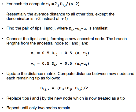 아래 그림은 NJ의 한예이다. 아래 그림의 왼쪽 상단의 table과 같이 distance matrix가 주어졌다고 할때 오른쪽 상단의 table과 같이 u 값을 계산한다. 그 뒤 왼쪽 하단과 같은 새로운 distance matrix를 생성하고 이 값중 제일 작은 값을 갖는 pair를 찾는다(-39가 가장 작은 값으로 A,B 와 C,D가 있는데 여기서는 C,D를 선택). 그뒤 오른쪽 하단과 같이 새로운 노드 X와 C,D의 거리를 구한다.
 C와 D가 clustering 되어 새로운 노드 X를 생성한 뒤 아래 그림과 같이 새로운 X 노드와 나머지 노드 간의 거리를 구해야 한다.
 C,D의 record는 삭제한 뒤 A,B,X 만 가지고 위 과정을 반복한다. 최종적으로 아래와 같은 그림으로 완성

-----------------------------------------------------------------
%정리를 하자면 tree를 구축하는 방식은 exhaustive, branch and bound, 그리고 heuristic 방식이 있는 것. 그리고 그 tree를 평가 하는 방식으로 maximum parsimony, distance matrix method가 있는 것. maximum parsimony의 경우 fitch algorithm으로 계산 가능하고, distance matrix의 경우 tree 선택 기준에 least squares 와 minimum evolution 방식으로 나눌 수 있다.
추가적으로 matrix distance method의 경우에는 clustering 방식으로 optimal tree를 결정할 수 있는데 NJ(neighbor joining algorithm)이 그 한 방법이다. NJ 방법은 distance matrix에서 가장 짧은 노드를 합치는 식으로 step-by-step으로 phylogenetic tree를 구축하는 방법이다.
https://class.coursera.org/molevol-001/class/index
https://spark-public.s3.amazonaws.com/molevol/Downloads/slides_week1.pdf
... (1~6 까지)
아래 내용은 단순히 위 URL의 vod를 요약한 것으로 추가적인 자료 확인이나 이해를 높이기 위한 노력이 없었으므로 잘못된 해석이 들어가 있을 수 있다.
또한 강의 초반의 classification, evolution, selection, genetic drift, phylogenetic tree teminology 등은 생략한다.
molecular data, 즉 DNA sequence로 부터 어떻게 phylogenetic tree를 구축하는지 알아본다.
<Maximum Parsimony>
simplest possible hypothesis를 선택하는 것이 maximum parsimony 방식. 곧 shortest tree(데이터를 나타내는데 필요한 mutation 갯수가 가작 적은 tree) 를 선택하는 방식.


위의 tree는 3개의 bp를 모두 고려 했을때의 tree length를 나타낸 것으로 위의 maximum parsimony의 방식으로는 tree가 적당한 tree로 판단된다.
다르게 표현하면 maximum parsimony는 homoplasy가 가장 적게 나타나는 tree를 선택하는 것이다.

그러면 DNA 데이터로 부터 어떻게 maximum parsimony tree를 찾을까? (이 수업에서는 DNA의 multiple alignment에 대해서는 설명하지 않음)
아래와 같은 순서대로 parsiminious tree를 찾음
1. Construct list of all possible trees for data set
2. For each tree: determine length, add to list of lengths
3. When finished: select tree from list
4. If several trees have the same length, then they are equally good (equally parsimonious)
tree를 construction 하는 방법은 아래와 같다(이 같은 방식을 exhaustive search 라고 함, 모든 tree를 다 찾는 방식).

tree가 구축되었으면 그 다음 tree length를 구하는 방법이 필요. 그것이 fitch algorithm.
<The Fitch Algorithm>
1. Root the tree at an arbitrary internal node (or internal branch)
2. Visit an internal node x for which no state set has been defined, but where the state sets of x's immediate descentdants (y,z) have been defined
3. If the state sets of y,z have common states, then union of y,z to x, and increase tree length by one
4. Repeat until all internal nodes have been visited. Note length of current tree.

모든 tree를 다 구축해보는 것은 현실적으로 불가능. 이에 대한 방안을 알아본다.
<Searching Tree Space>
exhaustive search는 엄청나게 많은 tree를 생성하게 된다(위의 exhaustive search의 그림과 아래 table 참고).

그 대안으로 나온것이 Branch and bound 방식. 랜덤하게 tree 하나를 뽑아서 그것의 length를 구하고 그것을 기준으로 삼는것. 그래서 tree construction 할때 그 기준보다 넘어가버리면 아예 그것과 관련된 tree는 더이상 계산하지 않는 것이다.

위 그림의 오른쪽 상단의 것을 기준으로 삼으면 tree를 construction 할때 두번째 layer의 오른쪽과 왼쪽의 tree는 이미 기준의 tree보다 length가 길기 때문에 더이상 샘플을 adding 하지 않는다.
하지만 branch and bound 역시 샘플 수가 많으면 효과적인 방법이 아님.
그래서 나온방식이 Heuristic search.
1.Construct initial tree (e.g.,sequential addition); determine length
2. Construct set of "neighboring trees" by making small rearrangements of initial tree; determine lengths
3.If any of the neighboring trees are better than the initial tree, then select it/them and use as starting point for new round of rearrangements (possibly several neighbors are equally good)
4. Repeat steps 2+3 until you have found a tree that is better than all of its neighbors
5. This tree is a "local optimum" (not necessarily a global optimum)
랜덤하게 tree 하나 뽑아서 length 구하고 이 tree의 rearrangement 해서 length를 구하고 이 새로운 tree가 기존의 tree 보다 length가 짧아지면 이 tree로 갈아타서 또 rearrange 하고.. 이를 반복해서 local optimum을 찾는것. 곧 경험적으로 해봐서 더이사 좋아지지 않는다 싶으면 멈추는 것을 의미.
tree의 rearrangement는 아래와 같이 3가지 방식이 있다. TBR > SPR > NNI


maximum parsimony 같은 방법을 이용하면 equally parsimonious 한 tree들이 많이 찾아지게 된다. 이때 어떻게 해야 하는가? 여기서 어떠한 정보를 뽑아 낼 수 있는가?
<consensus tree>
설령 수많은 equally parsimonious trees 가 찾아졌다 하더라도 실상 tree들의 전체 적인 형태는 비슷하며 단지 약간의 차이가 있을 뿐이다. 그렇기 때문에 consensus tree를 구축함으로써 tree set으로부터 정보를 뽑아 낼수 있다.

위와 같이 strict consensus tree는 모호한 부분은 polytomy를 이용하여 나타내는 방법 (첫번째와 두번째 tree는 동일한데, 어떻게 동일한 tree가 두번 나올수 있냐에 대해서는 저 tree들이 더 큰 tree의 subtree라고 가정해보면 됨).

majority consensus tree를 구축하는 방법
1. tree set의 tree 하나씩 모든 internal branch를 기준으로 bipartition으로 해서 나타나는 separation을 table로 정리한다.
2. 정리되 table을 count를 frequency로 바꾼뒤 ordering 해서 50이상의 값을 갖는 separation을 찾는다.


maximum parsimony 이외에 DNA data를 잘 나타내는 phylogenetic tree를 찾는 방법을 알아본다.
<Distance Matrix Method>


distance matrix method 역시 parsimony와 같이 tree를 만들어 놓고 평가하는 방식이다. 그렇기 때문에 tree가 많아지면 exhaustive method 방식보다는 heuristic algorithm을 이용하여 효율을 높일 수 있다. distance matrix method의 경우 이 외에도 clustering algorithm 을 이용할 수 있는데 그 한 방법인 neighbor joining 방법을 알아본다.
Neighbor Joining(NJ) Agorithm
알고리즘은 아래와 같다.


-----------------------------------------------------------------
%정리를 하자면 tree를 구축하는 방식은 exhaustive, branch and bound, 그리고 heuristic 방식이 있는 것. 그리고 그 tree를 평가 하는 방식으로 maximum parsimony, distance matrix method가 있는 것. maximum parsimony의 경우 fitch algorithm으로 계산 가능하고, distance matrix의 경우 tree 선택 기준에 least squares 와 minimum evolution 방식으로 나눌 수 있다.
추가적으로 matrix distance method의 경우에는 clustering 방식으로 optimal tree를 결정할 수 있는데 NJ(neighbor joining algorithm)이 그 한 방법이다. NJ 방법은 distance matrix에서 가장 짧은 노드를 합치는 식으로 step-by-step으로 phylogenetic tree를 구축하는 방법이다.
Subscribe to:
Posts (Atom)